रिटेल Demand Forecasting: Sales History से बेहतर Reorder Decision

कल्पना करें कि शुक्रवार को तीन दुकानों वाले homeware retailer की लोकप्रिय kettle बिक चुकी है, मगर stockroom में 140 candle holders पड़े हैं। Supplier को अगली delivery के लिए दो हफ्ते चाहिए। यह समझाने का दृश्य है, किसी वास्तविक ग्राहक का परिणाम नहीं।

पुरानी reorder setting तब की है जब kettle सप्ताह में 30 बिकती थी; अब team को कहीं अधिक run rate दिख रहा है। हर चीज़ ज़्यादा खरीदने से cash फँसेगा, निर्णय नहीं सुधरेगा। Demand, supplier timing और वास्तव में कितने अंतराल पर stock देखते हैं—तीनों समझने होंगे।

यह गाइड आठ सप्ताह की काल्पनिक SKU history से आसान forecast test और दो replenishment policies दिखाता है। सभी quantities शिक्षण के अनुमान हैं। Formulas तभी उपयोगी हैं जब assumptions काम से मेल खाएँ; शुक्रवार को कभी stockout न होने का वादा नहीं है। समीक्षा: 4 नवंबर 2026।

किस Demand की Planning है, तय करें

पहले SKU, location, unit, time bucket और horizon तय करें। Sales पूरी हुई खरीद बताती हैं, ग्राहक जितना खरीदना चाहते थे वह सब नहीं। Stockout demand छिपा सकता है; zero-sale day अपने आप zero demand या निश्चित lost sale का प्रमाण नहीं। Availability, खुलने के समय और भरोसेमंद enquiry/lost-sale evidence देखें।

Observed sales, estimated lost demand और management override अलग रखें। Stockout estimate अनिश्चित है, sales ledger में जोड़ने वाला transaction नहीं। हर बड़ा order अपने आप न हटाएँ; देखें कि वह repeat customer, one-off event या अगले horizon का ज्ञात commitment है।

Outbound demand और वापसी से मिलने वाली usable supply अलग forecast करें। लौटी kettle देर से, खराब या बेचने योग्य न भी आए। Net sales वित्त में उपयोगी हैं, मगर हमेशा replenishment quantity नहीं। संबंधित अवधि में भरोसेमंद उपयोग योग्य returns ही supply में गिनें।

Adjustment का साफ़ Record रखें

तालिका में मूल teaching data है। Week 2 में पहचाना गया one-off हिस्सा 10 units इस baseline से हटाया गया है, वास्तविक stock consumption record से नहीं। Week 4 में provisional lost-demand estimate 7 units है। मानें कि annotations उसी सप्ताह के अंत तक उपलब्ध थे; बाद की जानकारी से इन्हें बनाने पर backtest दूषित होगा।

Week	Recorded Units	Baseline Adjustment	Planning Series
1	44	0	44
2	71	−10: पहचाना one-off	61
3	52	0	52
4	31	+7: provisional lost demand	38
5	55	0	55
6	49	0	49
7	63	0	63
8	38	0	38

Recorded sales 403, adjusted series 400 और आठ सप्ताह का mean 50 है। Total समान दिखने से weekly timing सही नहीं सिद्ध होती। हर adjustment का कारण, evidence, तारीख और owner रखें तथा lost-demand के दूसरे अनुमान भी जाँचें।

Promotion और price change को flag करें, चुपचाप हटाएँ नहीं। Trend और calendar effect का उचित baseline चाहिए। Monthly seasonal ratio growth को seasonality मान सकता है या seasonal model का effect दो बार जोड़ सकता है। अधिक repeated cycles मदद करते हैं, मगर दो साल से विश्वसनीय seasonality पक्की नहीं होती। बदलती तारीख वाले त्योहार और नए products पर विशेष ध्यान दें।

भविष्य की जानकारी के बिना Forecast Test

Four-week moving average समझाने योग्य candidate है, स्वतः सबसे अच्छा नहीं। Test week के पहले चार planning values ही लें। समान तारीख और जानकारी पर उचित naïve/seasonal baseline से तुलना करें। Stock decision दो या तीन सप्ताह का है तो उस horizon का cumulative forecast भी test करें।

यह one-week rolling example हिसाब समझाता है। चार test observations से production reliability सिद्ध नहीं होती। Forecast जैसा बनाया था वैसा version रखें; बाद में मिली जानकारी से उसके पुराने inputs न बदलें।

Week	Forecast	Actual Planning Value	Actual − Forecast	Absolute Error
5	48.75	55	+6.25	6.25
6	51.50	49	-2.50	2.50
7	48.50	63	+14.50	14.50
8	51.25	38	-13.25	13.25
कुल	200.00	205	+5.00	36.50

Week 8 के बाद पिछले चार सप्ताह का mean Week 9 के लिए 51.25 देगा, 50 नहीं। नीचे stock-policy उदाहरण में पूरे आठ सप्ताह से stationary planning mean 50 अलग assumption है। यह अलग सरल मॉडल है, latest moving-average forecast को 50 नहीं कहा गया।

Error Metrics की सीमाएँ भी समझें

इन चार सप्ताह की non-negative demand में WAPE = absolute errors का योग ÷ actuals का योग = 36.5 ÷ 205 = 17.8%। Denominator zero हो तो N/A दें। Volume, trend और mix बदलने पर अलग periods की तुलना भ्रामक हो सकती है; aggregate व्यक्तिगत SKU छिपा सकता है।

Sign तय करें: bias = sum(forecast − actual) ÷ sum(actual) = (200 − 205) ÷ 205 = −2.4%, यानी यहाँ overall underforecast। Errors आपस में कट सकते हैं; MAE = 36.5 ÷ 4 = 9.125 units। Universal WAPE target की जगह service, waste और purchase cost भी देखें।

Rolling-origin tests के लिए Forecasting: Principles and Practice पढ़ें। Hyndman का WAPE note denominator और non-stationarity की सीमा समझाता है। Scaling baseline सार्थक हो तो MASE/RMSSE भी देखें।

Continuous या Weekly Review चुनें

Continuous Review: inventory position बदलने पर देखें और reorder point या उससे नीचे आने पर तय replenishment decision चालू करें। Point बताता है कब, कितनी units खरीदनी हैं यह नहीं। Quantity policy, open orders और approval के अलग नियम चाहिए।

Weekly Periodic Review: हर तय review पर order-up-to target तक पहुँचने की quantity निकालें। अगले review तक का समय और supplier lead time दोनों protect करें। Weekly calculation करने के लिए continuous threshold तक पहुँचने का इंतज़ार न करें।

सरल backorder model में inventory position = usable on-hand + confirmed on-order − backorders। यह physical shelf stock या available-to-promise के बराबर नहीं। Reservations और commitments demand model से मिलाएँ ताकि दो बार न गिनें। Damaged stock हटाएँ; देर से या अनिश्चित receipts को due date से परखें, हर open PO समय पर आने की धारणा न रखें। उदाहरण में अन्य commitments या shortages नहीं हैं।

Assumptions लिखकर Safety Buffer निकालें

सिर्फ teaching calculation में: weekly mean d = 50, fixed lead time L = 2 weeks, independent स्थिर weekly demand, sample standard deviation σ = √(644/7) = √92 ≈ 9.5917 और normal approximation। 95% cycle service target पर z ≈ 1.64485। समय की units समान रखें और whole-unit requirement ऊपर round करें।

Continuous review: SS = z × σ × √L ≈ 22.31, ऊपर round करके 23 units। ROP = d × L + SS = 100 + 23 = 123 units। यह model threshold है, guarantee या 95% unit fill rate नहीं।

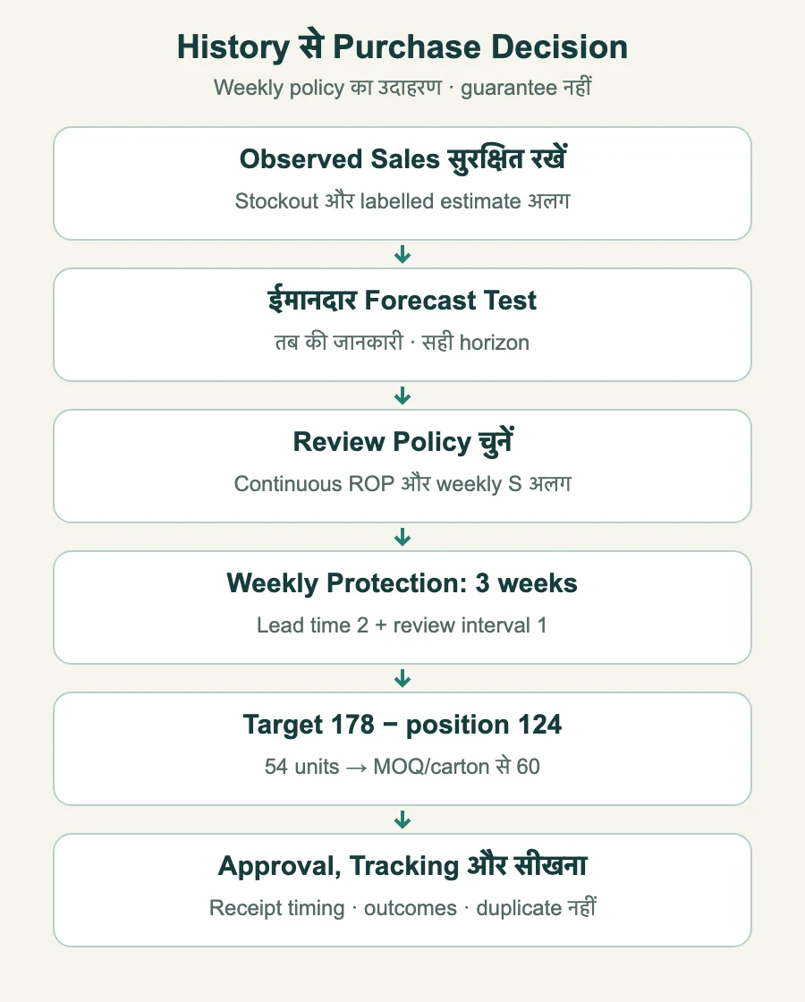
Weekly review में R = 1, इसलिए protection interval L + R = 3 weeks। Buffer z × σ × √3 ≈ 27.33, ऊपर round करके 28 units। Target S = 50 × 3 + 28 = 178 units। दो सप्ताह वाला buffer दोबारा लेने से इस model की protection कम आँकी जाएगी।

Weekly review में inventory position 124 हो तो q = max(0, 178 − 124) = 54। MOQ 60 और 12 की cartons होने पर 60 units order करें, cash, capacity, expiry और approval देखकर। Position 124 continuous ROP 123 से ऊपर है, फिर भी यह periodic order रद्द नहीं होता।

मानी गई Policy	Protection Interval	Rounded Buffer / Target
Continuous Review	2 weeks	SS 23 · ROP 123
Weekly Review	3 weeks	SS 28 · S 178

इसी continuous-review toy model में 90%, 95% और 99% cycle targets के rounded buffers 18, 23, 32 और reorder points 118, 123, 132 हैं। यहाँ ऊँचे target पर buffer बढ़ता है; उसका मूल्य shortage के नुकसान और holding cost पर है। ये theoretical inputs हैं, देखे गए service outcomes नहीं।

आठ adjusted observations normal और independent distribution सिद्ध नहीं करते। Seasonal, correlated, intermittent demand या variable lead time में actual protection interval के errors निकालें या उचित simulation करें। Supplier order से usable receipt तक का समय और uncertainty मापें; दो सप्ताह का average fixed दो सप्ताह का promise नहीं। लागू करने के बाद stockouts, fill rate और excess देखें।

Inventory concept और policy assumptions के लिए NC State safety-stock tutorial और Rossetti का continuous/periodic review अध्याय देखें। यहाँ हिसाब अलग से निकाला teaching example है।

Value, Variability और नुकसान से प्राथमिकता दें

ABC में value measure घोषित करें, जैसे annual usage cost, contribution या revenue। Threshold management choice है, अनिवार्य 80/15/5 नहीं। XYZ में CV = σ/mean variability बता सकता है, पर window, zero mean और seasonality की व्यवस्था चाहिए।

इस उदाहरण में CV ≈ 9.5917/50 = 0.192। स्थानीय X threshold इसे अपेक्षाकृत steady कह सकती है, पर इससे auto-purchase की अनुमति नहीं मिलती। कम revenue वाला spare भी critical हो सकता है और volatile item का stock ज़रूरी हो सकता है। CZ label के कारण ही product न हटाएँ।

Advanced Forecasting कब मदद करता है

निर्णय के समय उपलब्ध जानकारी पर complex model को विश्वसनीय simple baseline से तुलना करें। Promotion, price, substitute और product similarity मदद कर सकते हैं, नए items में भी; predictive value की guarantee नहीं। केवल SKU count से machine learning लेना या ठुकराना तय न करें।

निर्णय के लिए चुनें: out-of-sample horizon errors, service/waste, operating cost, explanation और exception handling। ज़रूरत हो तो location और aggregate plans मिलाएँ। StoreConsole का inventory module आवश्यक records और movement controls के लिए देखें; enabled forecasting और purchase-approval workflow अलग जाँचें। Low-stock alert या tour automatic forecasting engine का प्रमाण नहीं।

दोहराने योग्य Planning Routine

1. Evidence देखें। Stock और receipts मिलाएँ; stockouts, promotions, bulk commitments और provisional adjustments देखें। Raw history रखें।
2. Plan Refresh। Forecast version, horizon, assumptions और owner सुरक्षित रखें। तब उपलब्ध जानकारी लें और महत्वपूर्ण exceptions की uncertainty देखें।
3. Policy Review। चुना continuous/periodic rule लागू करें। Due receipts, usable stock और backorders बदलें; capacity, shelf life और buying constraints देखें।
4. Approve और Track। Proposed order जाँचें और reference, promised date व actual usable receipt लिखें। Timeout के बाद पहले पुराना reference देखें, ताकि retry duplicate purchase न बनाए।
5. नतीजों से सीखें। Bias, errors, missed demand, fills, waste और supplier reliability देखें। Assortment के अनुरूप cadence रखें; तीस मिनट या एक sign के तीन errors सार्वभौमिक नियम नहीं।

Kettle की Shelf पर लौटें

काल्पनिक दुकान का buyer अब observation, estimate और लागू purchase policy अलग समझता है। वह kettle order पर सवाल कर सकता है और candle holders का अलग फैसला ले सकता है। लाभ है दोहराने योग्य, audit करने योग्य decision; एक formula हर खाली shelf रोक देगा—यह वादा नहीं।

Anichur Rahaman StoreConsole के निर्माता हैं। गाइड operational planning समझाता है; दुकान की कहानी, demand values और service targets शिक्षण के उदाहरण हैं।